Message Passing Based Detection for Orthogonal Time Frequency Space Modulation
YUAN Zhengdao1, LIU Fei2, GUO Qinghua,3, WANG Zhongyong2
The Open University of Henan, Zhengzhou 450000, China
Zhengzhou University, Zhengzhou 450001, China
University of Wollongong, Wollongong NSW 2522, Australia
Received:2021-10-10
Fund supported:
the National Natural Science Foundation of China. 61901417. U1804152. 61801434 Science and Technology Research Project of Henan Province. 212102210556. 212102210566. 212400410179
About authors
YUAN Zhengdao received the B.E. degree in communication and information system from Henan University of Science and Technology, China in 2006, the M.E. degree in communication engineering from Soochow University, China in 2009, and the Ph.D. degree in information and communication engineering from the National Digital Switching System Engineering and Technological Research Center, China in 2018. He is currently an associate professor with the Open University of Henan. He was a visiting scholar with the University of Wollongong, Australia in 2019. His research interests are mainly in massive MIMO, sparse channel estimation, message passing algorithm, and iterative receiver.
LIU Fei received the B.E. and M.E. degrees in information and communication engineering from Zhengzhou University, China in 2015 and 2017, respectively. He is currently working toward the Ph.D. degree with the School of Information and Engineering, Zhengzhou University, China. His research interests are message passing algorithm, sparse signal recovery, and OTFS.
GUO Qinghua (qguo@uow.edu.au) received the B.E. degree in electronic engineering and the M.E. degree in signal and information processing from Xidian University, China in 2001 and 2004, respectively, and the Ph.D. degree in electronic engineering from the City University of Hong Kong, China in 2008. He is currently an associate professor with the School of Electrical, Computer and Telecommunications Engineering, University of Wollongong, Australia and an adjunct associate professor with the School of Engineering, The University of Western Australia. His research interests include signal processing, machine learning and telecommunications. He was a recipient of the Australian Research Council’s inaugural Discovery Early Career Researcher Award in 2012.
E-mail:qguo@uow.edu.au
WANG Zhongyong received the B.S. and M.S. degrees in automatic control from Harbin Shipbuilding Engineering Institute, China in 1986 and 1988, respectively, and the Ph.D. degree in automatic control theory and application from Xi’an Jiaotong University, China in 1998. From 1988 to 2002, he has been with the Department of Electronics, Zhengzhou University, China. Now he is a professor with the Department of Communication Engineering, Zhengzhou University. His research interests include numerous aspects within embedded systems, signal processing, and communication theory.
Abstract
The orthogonal time frequency space (OTFS) modulation has emerged as a promising modulation scheme for wireless communications in high-mobility scenarios. An efficient detector is of paramount importance to harvesting the time and frequency diversities promised by OTFS. Recently, some message passing based detectors have been developed by exploiting the features of the OTFS channel matrices. In this paper, we provide an overview of some recent message passing based OTFS detectors, compare their performance, and shed some light on potential research on the design of message passing based OTFS receivers.
YUAN Zhengdao, LIU Fei, GUO Qinghua, WANG Zhongyong. Message Passing Based Detection for Orthogonal Time Frequency Space Modulation. [J], 2021, 19(4): 34-44 doi:10.12142/ZTECOM.202104004
1 Introduction
Recently the orthogonal time frequency space (OTFS) modulation has attracted much attention due to its capability of achieving reliable communications in high mobility scenarios[1–6]. OTFS is a two-dimensional modulation scheme, and the information is modulated in the delay Doppler (DD) domain, which is in contrast to the time frequency (TF) domain modulation in the orthogonal frequency division multiplexing (OFDM). In OTFS, each symbol spreads over the time and frequency domains through the two dimensional (2D) inverse symplectic finite Fourier transform (SFFT), leading to both time and frequency diversities[1–2]. It has been shown that OTFS can significantly outperform OFDM in high mobility scenarios[7].
To harvest the diversities promised by OTFS, the design of a powerful detector is paramount. The optimal maximum a posteriori (MAP) detector is impractical due to its complexity growing exponentially with the length of the OTFS block. Recently, significant efforts have been devoted to the design of more efficient detectors. In Ref. [8], an effective channel matrix in the DD domain was derived, based on which a low-complexity two-stage detector was proposed. The first-order Neumann series was used in Ref. [9] to approximately solve the matrix inverse problem involved in the linear minimum mean squared error (MMSE) estimation based detection. A detection scheme was developed in Ref. [10], where the MMSE equalization was used in the first iteration, followed by parallel interference cancellation with a soft-output sphere decoder in subsequent iterations. A rectangular waveform was considered in Ref. [11], where the sparsity and quasi banded structure of channel matrices without fractional Doppler shifts were exploited to reduce the detection complexity. The linear equalizers were extended to the multiple input and multiple output (MIMO)-OTFS systems in Ref. [12]. A cross-domain method was proposed in Ref. [13], where a conventional linear MMSE estimator is adopted for equalization in the time domain and a low-complexity symbol-by-symbol detection is utilized in the DD domain. A low complexity iterative rake decision feedback detector was proposed in Ref. [14], which extracts and coherently combines the multiple copies of the symbols (due to multipath propagation) in the DD grid using maximal ratio combining (MRC).
Another line of OTFS detector design is based on factor graphs and message passing techniques[15, 23]. When the number of channel paths is small, the effective channel matrix in the DD domain is sparse, which allows efficient detection using the message passing algorithm (MPA)[2]. An expectation propagation (EP) algorithm was proposed in Ref. [16], where EP is used for message update with Gaussian approximation. A variational Bayes (VB) based detector was proposed in Ref. [17] to achieve better convergence. Studying the matched filtering processing, the authors in Ref. [18] proposed a message passing detector, which is combined with a probability clipping solution. The detectors in Refs. [2, 17, 19] take advantage of the sparsity of the channel matrix in the DD domain, and their complexity depends on the number of nonzero elements in each row of the channel matrix, which is denoted by . Without considering fractional Doppler shifts, is equal to the number of channel paths. In general, a wideband system can provide sufficient delay resolution. The Doppler resolution depends on the time duration of the OTFS block. To fulfill the low latency requirement in wireless communications, the time duration of an OTFS block should be relatively small, where it is necessary to consider fractional Doppler shifts[2, 20]. In this case, the value of can be significantly larger than the number of channel paths. In the case of rich scattering environments, the complexity of these detectors can be a concern and the short loops in the corresponding system graph model may result in significant performance. To overcome the above issues, the design of OTFS detectors based approximate message passing (AMP)[21–22] was investigated in Ref. [25]. AMP works well for independent and identically distributed (sub-)Gaussian system transfer matrix, but it suffers from performance loss or even diverges for a general system transfer matrix[27–29]. Instead, the works in Refs. [25–26] resort to the unitary AMP (UAMP)[27–29], which is a variant of AMP and was formerly called UTAMP[27]. In UAMP, a unitary transformation of the original model is used, where the unitary matrix for transformation can be the conjugate transpose of the left singular matrix of the general system transfer matrix[27] obtained through singular value decomposition (SVD). It is shown in Ref. [25] that UAMP is well suitable for OTFS due to the structure of block circulant matrix with circulant block (BCCB) of the DD domain channel matrices, where the 2D discrete Fourier transform is used for the unitary transformation, leading to very efficient implementation using the 2D fast Fourier transform (FFT) algorithm. In addition, as the noise variance is normally unknown, the noise variance estimation is also incorporated into the UAMP-based detector in Ref. [25].
In this paper, we provide an overview of the message passing based detectors, provide some comparison results, and discuss potential research on the design of message passing based OTFS receivers. The notations used in this paper are as follows. Boldface lower-case and upper-case letters denote vectors and matrices, respectively. We use and to denote the conjugate transpose and the transpose, respectively. The superscript denotes the conjugate operation. We define as the mod operation. We use to denote the probability density function of a complex Gaussian variable with mean and variance . The notation denotes the expectation of the function with respect to the distribution . The relation for some positive constant is written as . The notation represents the Kronecker product, and and represent the component-wise product and the division between vectors and , respectively. We use to denote that the vector is reshaped as an matrix column by column, where the length of is , and use to represent vectorization of matrix column by column. The notation represents a diagonal matrix with the elements of as its diagonal. We use to denote the element-wise magnitude squared operation for matrix . The notations and are used to denote an all-ones vector and an all-zeros vector with a proper length, respectively. The j-th entry of is denoted by . The superscript of denotes the iteration index of the variable s involved in an iterative algorithm.
2 System Model
The modulation and demodulation for OTFS are illustrated in Fig. 1, which are implemented with the 2D inverse SFFT (ISFFT) and SFFT at the transmitter and receiver, respectively[1, 24]. Before the OTFS modulation, a (coded) bit sequence is mapped to symbols , in the DD domain, where , is the cardinality of A, and denote the indices of the delay and Doppler shifts, respectively, and and are the number of grids of the DD plane. At the transmitter side, ISFFT is performed to convert the DD domain symbols to signals in the time-frequency (TF) domain.
Figure 1
Modulation and demodulation in an orthogonal time frequency space (OTFS) system[2]
.
After that, the signals in the TF domain are converted to a continuous-time waveform using the Heisenberg transform with a transmit waveform [2], i.e.,
,
where is subcarrier spacing and . Then the signal is transmitted over a time-varying channel and the received signal in the time domain is given as:
,
where is the channel impulse response in the continuous DD domain, and it can be expressed as[1]:
,
with being the Dirac delta function, being the number of channel paths, and , and being the gain, delay and Doppler shift associated with the i-th path, respectively. The delay and Doppler-shift taps for the i-th path are given by
, ,
where and are the delay and Doppler indices of the i-th path, and is a fractional Doppler associated with the i-th path. In the above equation, is the system bandwidth and is the duration of an OTFS block.
At the receiver, a receive waveform is used to transform the received signal to the TF domain, i.e.,
,
which is then sampled at and , yielding . Then SFFT is applied to to generate the DD domain signal , i.e.,
.
Assuming that the transmitted waveform and the received waveform satisfy the bi-orthogonal property[1], in the DD domain we have the input-output relationship[2].
,
where is an integer, and is the noise in the DD domain. We can see that for each path, the transmitted signal is circularly shifted, and scaled by a corresponding channel gain. We arrange {} as a vector , where the j-th element is with . Similarly, a vector can also be constructed based on . Then Eq. (8) can be rewritten in a vector form as:
,
where is the effective channel matrix in the DD domain, and denotes a white Gaussian noise with mean 0 and variance (or precision ). The channel matrix in Eq. (9) can be represented as[25]:
,
where denotes an matrix obtained by circularly shifting the rows of the identity matrix by , and is obtained similarly. Without fractional Doppler, i.e., , the channel matrix is reduced to
.
3 Message Passing (MP) Based Detectors
Based on the model (9) in the DD domain, several detectors have been proposed using the message passing techniques.
In model (9), the DD domain complex channel matrix is sparse (especially in the case without fractional Doppler shifts), which makes belief propagation suitable for implementing the OTFS detectors. In Eq. (2), and are length-MN complex vectors with elements denoted by and , , the element of is denoted by , , is a length-MN symbol vector with elements , , and denotes the modulation alphabet.
Thanks to the sparsity of , the joint distribution of the random variables in model (9) can be represented with a sparsely-connected factor graph with variable nodes corresponding to and observation nodes corresponding to . As shown in Fig. 2, each observation node is connected to a set of variable nodes , and similarly, each variable node is connected to a set of observation nodes , where and respectively denote the sets of indexes of non-zero elements in the d-th row and c-th columns of , and . The probability mass function (PMF) represents the messages from variable nodes to factor nodes .
Figure 2
Graph representation used to derive the message passing (MP) detector in Ref. [2]
Based on the factor graph in Fig. 2, a message passing algorithm was proposed in Ref. [2], and the detector is called MP detector in this paper. The following is a brief derivation of the message computations in the i-th iteration of the message computations.
1) Messages passing from observation node to variable node
The message is approximated to be Gaussian, and the mean and variance are computed as
,
.
2) Messages passing from variable node to observation node
The PMF can be updated as
,
where is the damping factor and
,
with
.
After a certain number of iterations by repeating 1) and 2), the decision on the transmitted symbol can be obtained, i.e.,
Output: The decision on transmitted symbols using Eq. (17)
The MP algorithm shown above is an approximation to loopy belief propagation since it approximates the interference to be Gaussian to achieve lower complexity. The complexity of the algorithm is per iteration, which depends on the sparsity of the channel, i.e., the value of S. When S is small, the detector is very attractive because it has low complexity and the detector delivers a good performance as no short loops in the factor graph model. However, in the case of rich-scatting environments and fractional Doppler shifts, the value of S can be large, leading to a denser factor graph model, which can affect the performance of the MP detector and result in a significant increase in computational complexity.
3.2 VB Detector
The VB detector was proposed in Ref. [17] to guarantee the convergence of the iterative detector, which can be implemented with variational message passing. With model (9), the optimal MAP detection can be formulated as:
.
However, the complexity of solving the above optimization problem increases exponentially with the size of . VB is adopted to achieve low complexity approximate detection. In this method, a distribution from a tractable distribution family is found as an approximation to the a posteriori distribution . The trial distribution can be obtained by minimizing the Kullback-Leibler divergence , i.e.,
,
where the expectation is taken over according to the trial distribution .
To simplify the optimization problem, q(x) is assumed to be fully factorized, i.e.,
,
where , and denotes the -th entry of . With this assumption, can be updated iteratively by maximizing . Since the noise sample and data symbol , are independent, and , can be rewritten as:
,
where , denotes the equivalent channel vector whose -th entry is . Then the distribution can be further rewritten as:
,
where
,
,
with , , and . Substituting in Eq. (23) and into yields
.
To find a stationary point of , the partial derivations of with respect to all local functions , need to be zero. Take the latent variable as an example. Setting the partial derivation to zero leads to:
,
where , is obtained in the -th iteration and denotes a constant.
Then, solving Eq. (27) for results in the local distribution, which can be expressed as:
,
where .
It is noted that the variance of is underestimated and only the noise variance is considered in Eq. (28). To fix the underestimation, a practical solution is to repeat the above procedure to approximate the a posteriori distribution for all the data symbols iteratively, resulting in the approximate marginal ,. Then, the decision on the symbols can be made by maximizing the approximate marginal distribution , i.e.,
.
The complexity of the algorithm per iteration is .
3.3 UAMP Detector
Leveraging the UAMP algorithm, the UAMP detector was developed in Ref.[25], where the BCCB structure of the DD domain channel matrix is exploited, leading to a highly efficient OTFS detector with 2D FFT. It can be seen from Eqs. (10) and (11) that the DD domain channel matrix has a BCCB structure. A useful property of the BCCB matrix is that it can be diagonalized using 2D Discrete Fourier Transform matrix, i.e.,
,
where with and being respectively the normalized -point and -point DFT matrices. In Eq. (30), matrix is a diagonal matrix, i.e.,, and is a length- vector that can be computed using 2D FFT.
,
where represents the 2D FFT operation, is an matrix, and with length- is the first column of matrix .
The above property is exploited in the design of the UAMP detector, leading to high computational efficiency while with outstanding performance compared with the existing detectors. Instead of using model (9) directly, the UAMP algorithm[27–29] works with the unitary transform of the model. The channel matrix admits the diagonalization in Eq. (30), leading to the following unitary transform of the OTFS system model:
,
where , , and the noise has the same distribution with as is an unitary matrix. The precision of the noise is still denoted by , which needs to be estimated. Define and an auxiliary vector . Then we can factorize the joint distribution of the unknown variables given as
,
where indices . To facilitate the factor graph representation of the factorization in Eq. (33), the relevant notations are listed in Table 1, which shows the correspondence between the factor nodes and their associated distributions. The factor graph representation for the factorization in Eq. (33) is depicted in Fig. 3.
Table 1
Table 1Factors, underlying distributions and functional forms associated with Eq. (31)
Following the UAMP algorithm, a UAMP based iterative detector can be designed, which is summarized in Algorithm 2. According to the derivation of (U)AMP using loopy belief propagation, UAMP provides the message from variable node to function node , which is Gaussian and denoted by . Here, the mean and the variance are given in Lines 1 and 2 of the Algorithm in a vector form. With the mean field rule[23] at the function node , we can compute the message passed from function node to variable node , i.e.,
,
where is the belief of . It turns out that is also Gaussian with its variance and mean given by
, ,
respectively, where is the estimate of in the last iteration. They can be expressed in a vector form shown in Lines 3 and 4 in Algorithm 2. The estimate of can be obtained based on the belief at the variable node shown in Fig. 3, i.e.,
.
And the estimate is given as
,
which can be rewritten in a vector form shown in Line 5 of the algorithm. With the mean field rule at the function node again, the message passed from the function node to the variable node can be computed as:
.
Then the UAMP algorithm with known noise can be used as if the true noise precision is , leading to Lines 6–15 and Lines 1–2 of the Algorithm 2. In Lines 10–13, the Gaussian message is combined with the discrete prior to obtain the MMSE estimates of the symbols in terms of their posterior means and variances. There is an extra operation in Line 14, which averages the variances of . Thanks to the special form of the unitary matrix , 2D FFT is used in the implementations in Lines 2 and 9. It can be seen that the UAMP detector does not require any matrix-vector products, the algorithm requires only element-wise vector operations or scalar operations, except Lines 2 and 9, which are implemented with FFT. So the complexity of the UAMP detector is per OTFS block per iteration, which is independent of .
Algorithm 2. UAMP detector for OTFS
Unitary transform: with . Calculated with Eq. (29), and define vector .
Initialize , , , , and .
Input: ,
Repeat
1:
2:
3:
4:
5:
6:
7:
8:
9:
10:
11:
12:
13:
14:
15:
Until terminated
Output: the estimate of i.e.,
Compared with the UAMP detector, the MP and VB detectors have a complexity of per OTFS block per iteration, which can be considerably higher than that of the UAMP detector in the case of rich scattering environments and when fractional Doppler shifts have to be considered (leading to a large ). Moreover, the UAMP detector can deliver much better performance when the number of paths is relatively large. In particular, the UAMP detector with estimated noise precision can significantly outperform other detectors with perfect noise precision. We note that, the OTFS detector can be implemented directly with the AMP algorithm. However, due to the deviation of the channel matrix from the i.i.d. Gaussian matrix, the AMP detector may perform poorly.
4 Turbo Processing in Coded Systems
It is well known that joint decoding and detection can bring significant system performance improvement, and it can be realized in a way that the detector and decoder exchange information iteratively, i.e., the turbo processing[30–31]. The OTFS detectors can be incorporated into a turbo receiver by endowing the OTFS detectors with the capabilities of taking the output log-likelihood ratios (LLRs) of the decoder as (soft) input and producing (soft) output in the form of extrinsic LLRs of the coded bits, i.e., the so-called soft input soft output (SISO) detector.
A typical turbo system is shown in Fig. 4, where and represent interleaver and de-interleaver, respectively. The information bits are encoded and interleaved before symbol mapping, where each symbol in the DD domain is mapped from a sub-sequence of the coded bit sequence, which is denoted by . Each corresponds to a length- binary sequence, which is denoted by . Based on the LLRs provided by the SISO decoder and the output of the OTFS demodulator as shown in Fig. 4, the task of the SISO OTFS detector is to compute the extrinsic LLR for each coded bit, i.e.,
Figure 4
Iterative joint detection and decoding in a coded OTFS system[25]
where is the output extrinsic LLR of the decoder in the last iteration. The extrinsic LLR is passed to the decoder. The extrinsic LLR can be expressed in terms of extrinsic mean and variance of the symbols[32], i.e.,
,
where and are the extrinsic mean and variance of , and and represent the subsets of all corresponding to and , respectively. The extrinsic variance and mean are defined in Ref. [32].
,
where and are the a priori mean and variance of calculated based on the output LLRs of the SISO decoder[30] and and are a posteriori mean and variance of .
Taking the UAMP detector as an example, we show the incorporation of the OTFS detector into a turbo receiver. According to the derivation of the UAMP algorithm, we can find that and consist of the extrinsic means and variances of the symbols in as they are the messages passed from the observation side and do not contain the immediate a priori information about . Hence we have and . Then Eq. (40) can be readily used to compute the extrinsic LLRs of the coded bits. With the LLRs provided by the SISO decoder, one can compute the probability for each , which is no longer the “non-informative prior ” in Algorithm 2. Therefore, in Line 7 of the algorithm is changed to
.
In addition, the iteration of the UAMP detector can be combined with the iteration between the SISO decoder and detector, which leads to a single loop iteration (i.e., inner iterations are not required).
The computational complexity of the detectors is summarized in Table 2. In the above discussion, we focus on the bi-orthogonal waveform. The detectors can be extended to OTFS systems with other waveforms, such as the simple rectangular waveform[25].
Table 2
Table 2Computational complexity of various detectors per iteration
In this section, we compare the performance of the message passing based detectors. The low complexity MRC detector in Ref. [14] is also included. We set and , i.e., there are time slots and subcarriers in the TF domain. Both quadrature phase shift keying (QPSK) modulation and 16-quadrature amplitude modulation (QAM) are considered. The carrier frequency is 3 GHz, and the subcarrier spacing is 2 kHz. The speed of the mobile user is set to , leading to a maximum Doppler frequency shift index . We assume that the maximum delay index is =14. The Doppler index of the i-th path is uniformly drawn from the set and the delay index is in the range of excluding the first path (). We assume that the fractional Doppler is uniformly distributed within , and the channel coefficients are independently drawn from a complex Gaussian distribution with mean 0 and variance , where the normalized power delay profile with being 0 or 0.1. The maximum number of iterations is set to 15 for all iterative detectors. We note that, all detectors except the MRC detector require the noise variance. The UAMP detector performs noise precision estimation, while the other detectors (except the MRC detector) including the AMP detector assume perfect noise precision. We evaluate the performance of the detectors in a variety of scenarios including the bi-orthogonal and rectangular waveforms with integer or fractional Doppler shifts, and QPSK or 16-QAM for modulations. In addition, both uncoded and coded systems are evaluated.
Fig. 5 shows the BER performance of various detectors in the case of the bi-orthogonal waveform with different numbers of paths, where we assume no fractional Doppler shifts, i.e., . We also assume , and QPSK is used. From this figure, we can see that, the MP detector performs well when , but with the increase of , its performance becomes worse. The VB detector has a similar trend. The MRC detector performs similarly to the MP and VB detectors when P=6 and delivers better performance than the MP and VB detectors with larger P. The AMP and UAMP detectors perform well, where we can see that they enjoy the diversity gain and achieve better performance with the increase of . In all cases, the UAMP based detector delivers the best performance and significantly outperforms other detectors.
Figure 5
BER performance of detectors with bi-orthogonal waveform and integer Doppler shifts (results are based on Ref. [25])
With the rectangular waveform and factional Doppler shifts, we compare the bit error ratio (BER) performance of the AMP, UAMP and MRC detectors in Fig. 6, where the number of paths and is used for the power delay profile. Both QPSK and 16-QAM are considered. Due to the deviation of the channel matrix from the i.i.d. (sub-) Gaussian matrix, AMP exhibits performance loss, leading to significantly worse performance compared with the UAMP detector. Thanks to the robustness of UAMP against a general matrix, UAMP performs well. We can see that the MRC detector performs better than the AMP detector. The UAMP detector performs the best and the gaps between other detectors with the UAMP detector become larger in the case of higher order modulation 16-QAM, compared with QPSK.
Figure 6
BER performance of detectors with the rectangular waveform and fractional Doppler shifts (results are based on Ref. [25])
We then evaluate the performance of the detectors in a coded OTFS system, where the turbo receiver in Fig. 4 is employed. The number of paths P=14, and a rectangular waveform is used. In Fig. 7(a), we show the performance of the uncoded system with the AMP and UAMP detectors. In Fig. 7(b), we use a rate-1/2 convolutional code with a generator followed by a random interleaver and QPSK modulation. The length of the codeword is . The BCJR algorithm is used for the SISO decoder. We can find that the performance gaps between the AMP detector and the UAMP detector become larger in the coded system. The turbo receiver can achieve much better performance (about dB at the BER of ) thanks to the joint processing of decoding and detection. In Fig. 7(c), we investigate the performance of the system with a more powerful LDPC. The 8 192 information bits are coded at rate R=1/2 by an irregular LDPC code with an average column weight of 3, then the coded bits are randomly interleaved and mapped. As expected, the system performance is improved considerably when the LDPC is used. From Fig. 7(c), we can see that the use of the LDPC code can improve the performance of the UAMP based detector significantly and the performance gap between AMP and UAMP increases when the LDPC is used.
Figure 7
BER performance comparison of coded and uncoded system with rectangular waveform (part of the results is based on Ref. [25])
6 Conclusions and Potential Future Work
In this paper, we review and compare the recently proposed message passing based OTFS detectors, which exploit the structures of the OTFS channel matrices, such as sparsity and BCCB. According to the results, the MP and VB detectors are more suitable in the scenarios that the number of paths is relatively small and the modulation order is low, where they deliver good performance while with relatively low complexity. The UAMP detector seems very promising especially in the case of rich-scattering environments and/or when fractional Doppler shifts have to be considered, where the UAMP detector is attractive in both computational complexity and performance. The results also show that the OTFS system with a turbo receiver can provide significant performance gain.
The message passing techniques seem promising in the design of OTFS receivers. In this paper, we assume the OTFS channel matrix is known, which however has to be estimated for practical applications. Message passing based OTFS channel estimation has been investigated in the literature, such as the work in Ref. [33]. With the message passing techniques, channel estimation and detection can be integrated for joint channel estimation and detection, which is expected to lead to superior system performance and/or significant reduction of the training overhead. This is because the data symbols can be used to serve as a virtual training sequence and the guard band between the training symbols and data symbols is not necessary.
It has been shown that joint decoding and detection based on a turbo receiver can significantly improve the system performance. The system performance can be potentially further improved by optimizing the error control codes. This requires fast and accurate performance prediction of the iterative receiver, so that the error control codes, e.g., LDPC, can be optimized.
The message passing techniques could be used to implement sophisticated receivers in more complex systems, such as multi-user OTFS systems, grant-free multiple access with OTFS, multiple-output-multiple-input (MIMO)-OTFS, integrated sensing and communication with OTFS.
... Recently the orthogonal time frequency space (OTFS) modulation has attracted much attention due to its capability of achieving reliable communications in high mobility scenarios[1–6]. OTFS is a two-dimensional modulation scheme, and the information is modulated in the delay Doppler (DD) domain, which is in contrast to the time frequency (TF) domain modulation in the orthogonal frequency division multiplexing (OFDM). In OTFS, each symbol spreads over the time and frequency domains through the two dimensional (2D) inverse symplectic finite Fourier transform (SFFT), leading to both time and frequency diversities[1–2]. It has been shown that OTFS can significantly outperform OFDM in high mobility scenarios[7]. ...
... [1–2]. It has been shown that OTFS can significantly outperform OFDM in high mobility scenarios[7]. ...
... The modulation and demodulation for OTFS are illustrated in Fig. 1, which are implemented with the 2D inverse SFFT (ISFFT) and SFFT at the transmitter and receiver, respectively[1, 24]. Before the OTFS modulation, a (coded) bit sequence is mapped to symbols , in the DD domain, where , is the cardinality of A, and denote the indices of the delay and Doppler shifts, respectively, and and are the number of grids of the DD plane. At the transmitter side, ISFFT is performed to convert the DD domain symbols to signals in the time-frequency (TF) domain. ...
... where is the channel impulse response in the continuous DD domain, and it can be expressed as[1]: ...
... Assuming that the transmitted waveform and the received waveform satisfy the bi-orthogonal property[1], in the DD domain we have the input-output relationship[2]. ...
Interference cancellation and iterative detection for orthogonal time frequency space modulation
11
2018
... Recently the orthogonal time frequency space (OTFS) modulation has attracted much attention due to its capability of achieving reliable communications in high mobility scenarios[1–6]. OTFS is a two-dimensional modulation scheme, and the information is modulated in the delay Doppler (DD) domain, which is in contrast to the time frequency (TF) domain modulation in the orthogonal frequency division multiplexing (OFDM). In OTFS, each symbol spreads over the time and frequency domains through the two dimensional (2D) inverse symplectic finite Fourier transform (SFFT), leading to both time and frequency diversities[1–2]. It has been shown that OTFS can significantly outperform OFDM in high mobility scenarios[7]. ...
... Another line of OTFS detector design is based on factor graphs and message passing techniques[15, 23]. When the number of channel paths is small, the effective channel matrix in the DD domain is sparse, which allows efficient detection using the message passing algorithm (MPA)[2]. An expectation propagation (EP) algorithm was proposed in Ref. [16], where EP is used for message update with Gaussian approximation. A variational Bayes (VB) based detector was proposed in Ref. [17] to achieve better convergence. Studying the matched filtering processing, the authors in Ref. [18] proposed a message passing detector, which is combined with a probability clipping solution. The detectors in Refs. [2, 17, 19] take advantage of the sparsity of the channel matrix in the DD domain, and their complexity depends on the number of nonzero elements in each row of the channel matrix, which is denoted by . Without considering fractional Doppler shifts, is equal to the number of channel paths. In general, a wideband system can provide sufficient delay resolution. The Doppler resolution depends on the time duration of the OTFS block. To fulfill the low latency requirement in wireless communications, the time duration of an OTFS block should be relatively small, where it is necessary to consider fractional Doppler shifts[2, 20]. In this case, the value of can be significantly larger than the number of channel paths. In the case of rich scattering environments, the complexity of these detectors can be a concern and the short loops in the corresponding system graph model may result in significant performance. To overcome the above issues, the design of OTFS detectors based approximate message passing (AMP)[21–22] was investigated in Ref. [25]. AMP works well for independent and identically distributed (sub-)Gaussian system transfer matrix, but it suffers from performance loss or even diverges for a general system transfer matrix[27–29]. Instead, the works in Refs. [25–26] resort to the unitary AMP (UAMP)[27–29], which is a variant of AMP and was formerly called UTAMP[27]. In UAMP, a unitary transformation of the original model is used, where the unitary matrix for transformation can be the conjugate transpose of the left singular matrix of the general system transfer matrix[27] obtained through singular value decomposition (SVD). It is shown in Ref. [25] that UAMP is well suitable for OTFS due to the structure of block circulant matrix with circulant block (BCCB) of the DD domain channel matrices, where the 2D discrete Fourier transform is used for the unitary transformation, leading to very efficient implementation using the 2D fast Fourier transform (FFT) algorithm. In addition, as the noise variance is normally unknown, the noise variance estimation is also incorporated into the UAMP-based detector in Ref. [25]. ...
... ] proposed a message passing detector, which is combined with a probability clipping solution. The detectors in Refs. [2, 17, 19] take advantage of the sparsity of the channel matrix in the DD domain, and their complexity depends on the number of nonzero elements in each row of the channel matrix, which is denoted by . Without considering fractional Doppler shifts, is equal to the number of channel paths. In general, a wideband system can provide sufficient delay resolution. The Doppler resolution depends on the time duration of the OTFS block. To fulfill the low latency requirement in wireless communications, the time duration of an OTFS block should be relatively small, where it is necessary to consider fractional Doppler shifts[2, 20]. In this case, the value of can be significantly larger than the number of channel paths. In the case of rich scattering environments, the complexity of these detectors can be a concern and the short loops in the corresponding system graph model may result in significant performance. To overcome the above issues, the design of OTFS detectors based approximate message passing (AMP)[21–22] was investigated in Ref. [25]. AMP works well for independent and identically distributed (sub-)Gaussian system transfer matrix, but it suffers from performance loss or even diverges for a general system transfer matrix[27–29]. Instead, the works in Refs. [25–26] resort to the unitary AMP (UAMP)[27–29], which is a variant of AMP and was formerly called UTAMP[27]. In UAMP, a unitary transformation of the original model is used, where the unitary matrix for transformation can be the conjugate transpose of the left singular matrix of the general system transfer matrix[27] obtained through singular value decomposition (SVD). It is shown in Ref. [25] that UAMP is well suitable for OTFS due to the structure of block circulant matrix with circulant block (BCCB) of the DD domain channel matrices, where the 2D discrete Fourier transform is used for the unitary transformation, leading to very efficient implementation using the 2D fast Fourier transform (FFT) algorithm. In addition, as the noise variance is normally unknown, the noise variance estimation is also incorporated into the UAMP-based detector in Ref. [25]. ...
... [2, 20]. In this case, the value of can be significantly larger than the number of channel paths. In the case of rich scattering environments, the complexity of these detectors can be a concern and the short loops in the corresponding system graph model may result in significant performance. To overcome the above issues, the design of OTFS detectors based approximate message passing (AMP)[21–22] was investigated in Ref. [25]. AMP works well for independent and identically distributed (sub-)Gaussian system transfer matrix, but it suffers from performance loss or even diverges for a general system transfer matrix[27–29]. Instead, the works in Refs. [25–26] resort to the unitary AMP (UAMP)[27–29], which is a variant of AMP and was formerly called UTAMP[27]. In UAMP, a unitary transformation of the original model is used, where the unitary matrix for transformation can be the conjugate transpose of the left singular matrix of the general system transfer matrix[27] obtained through singular value decomposition (SVD). It is shown in Ref. [25] that UAMP is well suitable for OTFS due to the structure of block circulant matrix with circulant block (BCCB) of the DD domain channel matrices, where the 2D discrete Fourier transform is used for the unitary transformation, leading to very efficient implementation using the 2D fast Fourier transform (FFT) algorithm. In addition, as the noise variance is normally unknown, the noise variance estimation is also incorporated into the UAMP-based detector in Ref. [25]. ...
... The modulation and demodulation for OTFS are illustrated in Fig. 1, which are implemented with the 2D inverse SFFT (ISFFT) and SFFT at the transmitter and receiver, respectively[1, 24]. Before the OTFS modulation, a (coded) bit sequence is mapped to symbols , in the DD domain, where , is the cardinality of A, and denote the indices of the delay and Doppler shifts, respectively, and and are the number of grids of the DD plane. At the transmitter side, ISFFT is performed to convert the DD domain symbols to signals in the time-frequency (TF) domain.
Modulation and demodulation in an orthogonal time frequency space (OTFS) system<sup>[<xref ref-type="bibr" rid="R2">2</xref>]</sup>
.
After that, the signals in the TF domain are converted to a continuous-time waveform using the Heisenberg transform with a transmit waveform [2], i.e., ...
... After that, the signals in the TF domain are converted to a continuous-time waveform using the Heisenberg transform with a transmit waveform [2], i.e., ...
... Assuming that the transmitted waveform and the received waveform satisfy the bi-orthogonal property[1], in the DD domain we have the input-output relationship[2]. ...
... Based on the model (9) in the DD domain, several detectors have been proposed using the message passing techniques.3.1 MP Detector in Ref. [<xref ref-type="bibr" rid="R2">2</xref>]
In model (9), the DD domain complex channel matrix is sparse (especially in the case without fractional Doppler shifts), which makes belief propagation suitable for implementing the OTFS detectors. In Eq. (2), and are length-MN complex vectors with elements denoted by and , , the element of is denoted by , , is a length-MN symbol vector with elements , , and denotes the modulation alphabet. ...
... Thanks to the sparsity of , the joint distribution of the random variables in model (9) can be represented with a sparsely-connected factor graph with variable nodes corresponding to and observation nodes corresponding to . As shown in Fig. 2, each observation node is connected to a set of variable nodes , and similarly, each variable node is connected to a set of observation nodes , where and respectively denote the sets of indexes of non-zero elements in the d-th row and c-th columns of , and . The probability mass function (PMF) represents the messages from variable nodes to factor nodes .
Graph representation used to derive the message passing (MP) detector in Ref. [<xref ref-type="bibr" rid="R2">2</xref>]
Based on the factor graph in Fig. 2, a message passing algorithm was proposed in Ref. [2], and the detector is called MP detector in this paper. The following is a brief derivation of the message computations in the i-th iteration of the message computations. ...
... Based on the factor graph in Fig. 2, a message passing algorithm was proposed in Ref. [2], and the detector is called MP detector in this paper. The following is a brief derivation of the message computations in the i-th iteration of the message computations. ...
... Algorithm 1. MPA detector in Ref. [2] ...
On the diversity of uncoded OTFS modulation in doubly-dispersive channels
0
2019
OTFS: A new generation of modulation addressing the challenges of
0
Performance analysis of coded OTFS systems over high-mobility channels
0
2021
Orthogonal time-frequency space modulation: a promising next-generation waveform
1
2021
... Recently the orthogonal time frequency space (OTFS) modulation has attracted much attention due to its capability of achieving reliable communications in high mobility scenarios[1–6]. OTFS is a two-dimensional modulation scheme, and the information is modulated in the delay Doppler (DD) domain, which is in contrast to the time frequency (TF) domain modulation in the orthogonal frequency division multiplexing (OFDM). In OTFS, each symbol spreads over the time and frequency domains through the two dimensional (2D) inverse symplectic finite Fourier transform (SFFT), leading to both time and frequency diversities[1–2]. It has been shown that OTFS can significantly outperform OFDM in high mobility scenarios[7]. ...
Low complexity modem structure for OFDM-based orthogonal time frequency space modulation
1
2018
... Recently the orthogonal time frequency space (OTFS) modulation has attracted much attention due to its capability of achieving reliable communications in high mobility scenarios[1–6]. OTFS is a two-dimensional modulation scheme, and the information is modulated in the delay Doppler (DD) domain, which is in contrast to the time frequency (TF) domain modulation in the orthogonal frequency division multiplexing (OFDM). In OTFS, each symbol spreads over the time and frequency domains through the two dimensional (2D) inverse symplectic finite Fourier transform (SFFT), leading to both time and frequency diversities[1–2]. It has been shown that OTFS can significantly outperform OFDM in high mobility scenarios[7]. ...
A simple two-stage equalizer with simplified orthogonal time frequency space modulation over rapidly time-varying channels
1
... To harvest the diversities promised by OTFS, the design of a powerful detector is paramount. The optimal maximum a posteriori (MAP) detector is impractical due to its complexity growing exponentially with the length of the OTFS block. Recently, significant efforts have been devoted to the design of more efficient detectors. In Ref. [8], an effective channel matrix in the DD domain was derived, based on which a low-complexity two-stage detector was proposed. The first-order Neumann series was used in Ref. [9] to approximately solve the matrix inverse problem involved in the linear minimum mean squared error (MMSE) estimation based detection. A detection scheme was developed in Ref. [10], where the MMSE equalization was used in the first iteration, followed by parallel interference cancellation with a soft-output sphere decoder in subsequent iterations. A rectangular waveform was considered in Ref. [11], where the sparsity and quasi banded structure of channel matrices without fractional Doppler shifts were exploited to reduce the detection complexity. The linear equalizers were extended to the multiple input and multiple output (MIMO)-OTFS systems in Ref. [12]. A cross-domain method was proposed in Ref. [13], where a conventional linear MMSE estimator is adopted for equalization in the time domain and a low-complexity symbol-by-symbol detection is utilized in the DD domain. A low complexity iterative rake decision feedback detector was proposed in Ref. [14], which extracts and coherently combines the multiple copies of the symbols (due to multipath propagation) in the DD grid using maximal ratio combining (MRC). ...
Low complexity iterative LMMSE-PIC equalizer for OTFS
1
2019
... To harvest the diversities promised by OTFS, the design of a powerful detector is paramount. The optimal maximum a posteriori (MAP) detector is impractical due to its complexity growing exponentially with the length of the OTFS block. Recently, significant efforts have been devoted to the design of more efficient detectors. In Ref. [8], an effective channel matrix in the DD domain was derived, based on which a low-complexity two-stage detector was proposed. The first-order Neumann series was used in Ref. [9] to approximately solve the matrix inverse problem involved in the linear minimum mean squared error (MMSE) estimation based detection. A detection scheme was developed in Ref. [10], where the MMSE equalization was used in the first iteration, followed by parallel interference cancellation with a soft-output sphere decoder in subsequent iterations. A rectangular waveform was considered in Ref. [11], where the sparsity and quasi banded structure of channel matrices without fractional Doppler shifts were exploited to reduce the detection complexity. The linear equalizers were extended to the multiple input and multiple output (MIMO)-OTFS systems in Ref. [12]. A cross-domain method was proposed in Ref. [13], where a conventional linear MMSE estimator is adopted for equalization in the time domain and a low-complexity symbol-by-symbol detection is utilized in the DD domain. A low complexity iterative rake decision feedback detector was proposed in Ref. [14], which extracts and coherently combines the multiple copies of the symbols (due to multipath propagation) in the DD grid using maximal ratio combining (MRC). ...
Low-complexity equalization for orthogonal time and frequency signaling (OTFS)
1
... To harvest the diversities promised by OTFS, the design of a powerful detector is paramount. The optimal maximum a posteriori (MAP) detector is impractical due to its complexity growing exponentially with the length of the OTFS block. Recently, significant efforts have been devoted to the design of more efficient detectors. In Ref. [8], an effective channel matrix in the DD domain was derived, based on which a low-complexity two-stage detector was proposed. The first-order Neumann series was used in Ref. [9] to approximately solve the matrix inverse problem involved in the linear minimum mean squared error (MMSE) estimation based detection. A detection scheme was developed in Ref. [10], where the MMSE equalization was used in the first iteration, followed by parallel interference cancellation with a soft-output sphere decoder in subsequent iterations. A rectangular waveform was considered in Ref. [11], where the sparsity and quasi banded structure of channel matrices without fractional Doppler shifts were exploited to reduce the detection complexity. The linear equalizers were extended to the multiple input and multiple output (MIMO)-OTFS systems in Ref. [12]. A cross-domain method was proposed in Ref. [13], where a conventional linear MMSE estimator is adopted for equalization in the time domain and a low-complexity symbol-by-symbol detection is utilized in the DD domain. A low complexity iterative rake decision feedback detector was proposed in Ref. [14], which extracts and coherently combines the multiple copies of the symbols (due to multipath propagation) in the DD grid using maximal ratio combining (MRC). ...
Low-complexity linear equalization for OTFS modulation
1
2020
... To harvest the diversities promised by OTFS, the design of a powerful detector is paramount. The optimal maximum a posteriori (MAP) detector is impractical due to its complexity growing exponentially with the length of the OTFS block. Recently, significant efforts have been devoted to the design of more efficient detectors. In Ref. [8], an effective channel matrix in the DD domain was derived, based on which a low-complexity two-stage detector was proposed. The first-order Neumann series was used in Ref. [9] to approximately solve the matrix inverse problem involved in the linear minimum mean squared error (MMSE) estimation based detection. A detection scheme was developed in Ref. [10], where the MMSE equalization was used in the first iteration, followed by parallel interference cancellation with a soft-output sphere decoder in subsequent iterations. A rectangular waveform was considered in Ref. [11], where the sparsity and quasi banded structure of channel matrices without fractional Doppler shifts were exploited to reduce the detection complexity. The linear equalizers were extended to the multiple input and multiple output (MIMO)-OTFS systems in Ref. [12]. A cross-domain method was proposed in Ref. [13], where a conventional linear MMSE estimator is adopted for equalization in the time domain and a low-complexity symbol-by-symbol detection is utilized in the DD domain. A low complexity iterative rake decision feedback detector was proposed in Ref. [14], which extracts and coherently combines the multiple copies of the symbols (due to multipath propagation) in the DD grid using maximal ratio combining (MRC). ...
Low-complexity linear MIMO-OTFS receivers
1
2021
... To harvest the diversities promised by OTFS, the design of a powerful detector is paramount. The optimal maximum a posteriori (MAP) detector is impractical due to its complexity growing exponentially with the length of the OTFS block. Recently, significant efforts have been devoted to the design of more efficient detectors. In Ref. [8], an effective channel matrix in the DD domain was derived, based on which a low-complexity two-stage detector was proposed. The first-order Neumann series was used in Ref. [9] to approximately solve the matrix inverse problem involved in the linear minimum mean squared error (MMSE) estimation based detection. A detection scheme was developed in Ref. [10], where the MMSE equalization was used in the first iteration, followed by parallel interference cancellation with a soft-output sphere decoder in subsequent iterations. A rectangular waveform was considered in Ref. [11], where the sparsity and quasi banded structure of channel matrices without fractional Doppler shifts were exploited to reduce the detection complexity. The linear equalizers were extended to the multiple input and multiple output (MIMO)-OTFS systems in Ref. [12]. A cross-domain method was proposed in Ref. [13], where a conventional linear MMSE estimator is adopted for equalization in the time domain and a low-complexity symbol-by-symbol detection is utilized in the DD domain. A low complexity iterative rake decision feedback detector was proposed in Ref. [14], which extracts and coherently combines the multiple copies of the symbols (due to multipath propagation) in the DD grid using maximal ratio combining (MRC). ...
Cross domain iterative detection for orthogonal time frequency space modulation
1
2021
... To harvest the diversities promised by OTFS, the design of a powerful detector is paramount. The optimal maximum a posteriori (MAP) detector is impractical due to its complexity growing exponentially with the length of the OTFS block. Recently, significant efforts have been devoted to the design of more efficient detectors. In Ref. [8], an effective channel matrix in the DD domain was derived, based on which a low-complexity two-stage detector was proposed. The first-order Neumann series was used in Ref. [9] to approximately solve the matrix inverse problem involved in the linear minimum mean squared error (MMSE) estimation based detection. A detection scheme was developed in Ref. [10], where the MMSE equalization was used in the first iteration, followed by parallel interference cancellation with a soft-output sphere decoder in subsequent iterations. A rectangular waveform was considered in Ref. [11], where the sparsity and quasi banded structure of channel matrices without fractional Doppler shifts were exploited to reduce the detection complexity. The linear equalizers were extended to the multiple input and multiple output (MIMO)-OTFS systems in Ref. [12]. A cross-domain method was proposed in Ref. [13], where a conventional linear MMSE estimator is adopted for equalization in the time domain and a low-complexity symbol-by-symbol detection is utilized in the DD domain. A low complexity iterative rake decision feedback detector was proposed in Ref. [14], which extracts and coherently combines the multiple copies of the symbols (due to multipath propagation) in the DD grid using maximal ratio combining (MRC). ...
Low complexity iterative rake decision feedback equalizer for zero-padded OTFS systems
2
2020
... To harvest the diversities promised by OTFS, the design of a powerful detector is paramount. The optimal maximum a posteriori (MAP) detector is impractical due to its complexity growing exponentially with the length of the OTFS block. Recently, significant efforts have been devoted to the design of more efficient detectors. In Ref. [8], an effective channel matrix in the DD domain was derived, based on which a low-complexity two-stage detector was proposed. The first-order Neumann series was used in Ref. [9] to approximately solve the matrix inverse problem involved in the linear minimum mean squared error (MMSE) estimation based detection. A detection scheme was developed in Ref. [10], where the MMSE equalization was used in the first iteration, followed by parallel interference cancellation with a soft-output sphere decoder in subsequent iterations. A rectangular waveform was considered in Ref. [11], where the sparsity and quasi banded structure of channel matrices without fractional Doppler shifts were exploited to reduce the detection complexity. The linear equalizers were extended to the multiple input and multiple output (MIMO)-OTFS systems in Ref. [12]. A cross-domain method was proposed in Ref. [13], where a conventional linear MMSE estimator is adopted for equalization in the time domain and a low-complexity symbol-by-symbol detection is utilized in the DD domain. A low complexity iterative rake decision feedback detector was proposed in Ref. [14], which extracts and coherently combines the multiple copies of the symbols (due to multipath propagation) in the DD grid using maximal ratio combining (MRC). ...
... In this section, we compare the performance of the message passing based detectors. The low complexity MRC detector in Ref. [14] is also included. We set and , i.e., there are time slots and subcarriers in the TF domain. Both quadrature phase shift keying (QPSK) modulation and 16-quadrature amplitude modulation (QAM) are considered. The carrier frequency is 3 GHz, and the subcarrier spacing is 2 kHz. The speed of the mobile user is set to , leading to a maximum Doppler frequency shift index . We assume that the maximum delay index is =14. The Doppler index of the i-th path is uniformly drawn from the set and the delay index is in the range of excluding the first path (). We assume that the fractional Doppler is uniformly distributed within , and the channel coefficients are independently drawn from a complex Gaussian distribution with mean 0 and variance , where the normalized power delay profile with being 0 or 0.1. The maximum number of iterations is set to 15 for all iterative detectors. We note that, all detectors except the MRC detector require the noise variance. The UAMP detector performs noise precision estimation, while the other detectors (except the MRC detector) including the AMP detector assume perfect noise precision. We evaluate the performance of the detectors in a variety of scenarios including the bi-orthogonal and rectangular waveforms with integer or fractional Doppler shifts, and QPSK or 16-QAM for modulations. In addition, both uncoded and coded systems are evaluated. ...
Factor graphs and the sum-product algorithm
1
2001
... Another line of OTFS detector design is based on factor graphs and message passing techniques[15, 23]. When the number of channel paths is small, the effective channel matrix in the DD domain is sparse, which allows efficient detection using the message passing algorithm (MPA)[2]. An expectation propagation (EP) algorithm was proposed in Ref. [16], where EP is used for message update with Gaussian approximation. A variational Bayes (VB) based detector was proposed in Ref. [17] to achieve better convergence. Studying the matched filtering processing, the authors in Ref. [18] proposed a message passing detector, which is combined with a probability clipping solution. The detectors in Refs. [2, 17, 19] take advantage of the sparsity of the channel matrix in the DD domain, and their complexity depends on the number of nonzero elements in each row of the channel matrix, which is denoted by . Without considering fractional Doppler shifts, is equal to the number of channel paths. In general, a wideband system can provide sufficient delay resolution. The Doppler resolution depends on the time duration of the OTFS block. To fulfill the low latency requirement in wireless communications, the time duration of an OTFS block should be relatively small, where it is necessary to consider fractional Doppler shifts[2, 20]. In this case, the value of can be significantly larger than the number of channel paths. In the case of rich scattering environments, the complexity of these detectors can be a concern and the short loops in the corresponding system graph model may result in significant performance. To overcome the above issues, the design of OTFS detectors based approximate message passing (AMP)[21–22] was investigated in Ref. [25]. AMP works well for independent and identically distributed (sub-)Gaussian system transfer matrix, but it suffers from performance loss or even diverges for a general system transfer matrix[27–29]. Instead, the works in Refs. [25–26] resort to the unitary AMP (UAMP)[27–29], which is a variant of AMP and was formerly called UTAMP[27]. In UAMP, a unitary transformation of the original model is used, where the unitary matrix for transformation can be the conjugate transpose of the left singular matrix of the general system transfer matrix[27] obtained through singular value decomposition (SVD). It is shown in Ref. [25] that UAMP is well suitable for OTFS due to the structure of block circulant matrix with circulant block (BCCB) of the DD domain channel matrices, where the 2D discrete Fourier transform is used for the unitary transformation, leading to very efficient implementation using the 2D fast Fourier transform (FFT) algorithm. In addition, as the noise variance is normally unknown, the noise variance estimation is also incorporated into the UAMP-based detector in Ref. [25]. ...
Low complexity receiver via expectation propagation for OTFS modulation
1
2021
... Another line of OTFS detector design is based on factor graphs and message passing techniques[15, 23]. When the number of channel paths is small, the effective channel matrix in the DD domain is sparse, which allows efficient detection using the message passing algorithm (MPA)[2]. An expectation propagation (EP) algorithm was proposed in Ref. [16], where EP is used for message update with Gaussian approximation. A variational Bayes (VB) based detector was proposed in Ref. [17] to achieve better convergence. Studying the matched filtering processing, the authors in Ref. [18] proposed a message passing detector, which is combined with a probability clipping solution. The detectors in Refs. [2, 17, 19] take advantage of the sparsity of the channel matrix in the DD domain, and their complexity depends on the number of nonzero elements in each row of the channel matrix, which is denoted by . Without considering fractional Doppler shifts, is equal to the number of channel paths. In general, a wideband system can provide sufficient delay resolution. The Doppler resolution depends on the time duration of the OTFS block. To fulfill the low latency requirement in wireless communications, the time duration of an OTFS block should be relatively small, where it is necessary to consider fractional Doppler shifts[2, 20]. In this case, the value of can be significantly larger than the number of channel paths. In the case of rich scattering environments, the complexity of these detectors can be a concern and the short loops in the corresponding system graph model may result in significant performance. To overcome the above issues, the design of OTFS detectors based approximate message passing (AMP)[21–22] was investigated in Ref. [25]. AMP works well for independent and identically distributed (sub-)Gaussian system transfer matrix, but it suffers from performance loss or even diverges for a general system transfer matrix[27–29]. Instead, the works in Refs. [25–26] resort to the unitary AMP (UAMP)[27–29], which is a variant of AMP and was formerly called UTAMP[27]. In UAMP, a unitary transformation of the original model is used, where the unitary matrix for transformation can be the conjugate transpose of the left singular matrix of the general system transfer matrix[27] obtained through singular value decomposition (SVD). It is shown in Ref. [25] that UAMP is well suitable for OTFS due to the structure of block circulant matrix with circulant block (BCCB) of the DD domain channel matrices, where the 2D discrete Fourier transform is used for the unitary transformation, leading to very efficient implementation using the 2D fast Fourier transform (FFT) algorithm. In addition, as the noise variance is normally unknown, the noise variance estimation is also incorporated into the UAMP-based detector in Ref. [25]. ...
A simple variational Bayes detector for orthogonal time frequency space (OTFS) modulation
3
2020
... Another line of OTFS detector design is based on factor graphs and message passing techniques[15, 23]. When the number of channel paths is small, the effective channel matrix in the DD domain is sparse, which allows efficient detection using the message passing algorithm (MPA)[2]. An expectation propagation (EP) algorithm was proposed in Ref. [16], where EP is used for message update with Gaussian approximation. A variational Bayes (VB) based detector was proposed in Ref. [17] to achieve better convergence. Studying the matched filtering processing, the authors in Ref. [18] proposed a message passing detector, which is combined with a probability clipping solution. The detectors in Refs. [2, 17, 19] take advantage of the sparsity of the channel matrix in the DD domain, and their complexity depends on the number of nonzero elements in each row of the channel matrix, which is denoted by . Without considering fractional Doppler shifts, is equal to the number of channel paths. In general, a wideband system can provide sufficient delay resolution. The Doppler resolution depends on the time duration of the OTFS block. To fulfill the low latency requirement in wireless communications, the time duration of an OTFS block should be relatively small, where it is necessary to consider fractional Doppler shifts[2, 20]. In this case, the value of can be significantly larger than the number of channel paths. In the case of rich scattering environments, the complexity of these detectors can be a concern and the short loops in the corresponding system graph model may result in significant performance. To overcome the above issues, the design of OTFS detectors based approximate message passing (AMP)[21–22] was investigated in Ref. [25]. AMP works well for independent and identically distributed (sub-)Gaussian system transfer matrix, but it suffers from performance loss or even diverges for a general system transfer matrix[27–29]. Instead, the works in Refs. [25–26] resort to the unitary AMP (UAMP)[27–29], which is a variant of AMP and was formerly called UTAMP[27]. In UAMP, a unitary transformation of the original model is used, where the unitary matrix for transformation can be the conjugate transpose of the left singular matrix of the general system transfer matrix[27] obtained through singular value decomposition (SVD). It is shown in Ref. [25] that UAMP is well suitable for OTFS due to the structure of block circulant matrix with circulant block (BCCB) of the DD domain channel matrices, where the 2D discrete Fourier transform is used for the unitary transformation, leading to very efficient implementation using the 2D fast Fourier transform (FFT) algorithm. In addition, as the noise variance is normally unknown, the noise variance estimation is also incorporated into the UAMP-based detector in Ref. [25]. ...
... , 17, 19] take advantage of the sparsity of the channel matrix in the DD domain, and their complexity depends on the number of nonzero elements in each row of the channel matrix, which is denoted by . Without considering fractional Doppler shifts, is equal to the number of channel paths. In general, a wideband system can provide sufficient delay resolution. The Doppler resolution depends on the time duration of the OTFS block. To fulfill the low latency requirement in wireless communications, the time duration of an OTFS block should be relatively small, where it is necessary to consider fractional Doppler shifts[2, 20]. In this case, the value of can be significantly larger than the number of channel paths. In the case of rich scattering environments, the complexity of these detectors can be a concern and the short loops in the corresponding system graph model may result in significant performance. To overcome the above issues, the design of OTFS detectors based approximate message passing (AMP)[21–22] was investigated in Ref. [25]. AMP works well for independent and identically distributed (sub-)Gaussian system transfer matrix, but it suffers from performance loss or even diverges for a general system transfer matrix[27–29]. Instead, the works in Refs. [25–26] resort to the unitary AMP (UAMP)[27–29], which is a variant of AMP and was formerly called UTAMP[27]. In UAMP, a unitary transformation of the original model is used, where the unitary matrix for transformation can be the conjugate transpose of the left singular matrix of the general system transfer matrix[27] obtained through singular value decomposition (SVD). It is shown in Ref. [25] that UAMP is well suitable for OTFS due to the structure of block circulant matrix with circulant block (BCCB) of the DD domain channel matrices, where the 2D discrete Fourier transform is used for the unitary transformation, leading to very efficient implementation using the 2D fast Fourier transform (FFT) algorithm. In addition, as the noise variance is normally unknown, the noise variance estimation is also incorporated into the UAMP-based detector in Ref. [25]. ...
... The VB detector was proposed in Ref. [17] to guarantee the convergence of the iterative detector, which can be implemented with variational message passing. With model (9), the optimal MAP detection can be formulated as: ...
A low-complexity message passing detector for OTFS modulation with probability clipping
1
2021
... Another line of OTFS detector design is based on factor graphs and message passing techniques[15, 23]. When the number of channel paths is small, the effective channel matrix in the DD domain is sparse, which allows efficient detection using the message passing algorithm (MPA)[2]. An expectation propagation (EP) algorithm was proposed in Ref. [16], where EP is used for message update with Gaussian approximation. A variational Bayes (VB) based detector was proposed in Ref. [17] to achieve better convergence. Studying the matched filtering processing, the authors in Ref. [18] proposed a message passing detector, which is combined with a probability clipping solution. The detectors in Refs. [2, 17, 19] take advantage of the sparsity of the channel matrix in the DD domain, and their complexity depends on the number of nonzero elements in each row of the channel matrix, which is denoted by . Without considering fractional Doppler shifts, is equal to the number of channel paths. In general, a wideband system can provide sufficient delay resolution. The Doppler resolution depends on the time duration of the OTFS block. To fulfill the low latency requirement in wireless communications, the time duration of an OTFS block should be relatively small, where it is necessary to consider fractional Doppler shifts[2, 20]. In this case, the value of can be significantly larger than the number of channel paths. In the case of rich scattering environments, the complexity of these detectors can be a concern and the short loops in the corresponding system graph model may result in significant performance. To overcome the above issues, the design of OTFS detectors based approximate message passing (AMP)[21–22] was investigated in Ref. [25]. AMP works well for independent and identically distributed (sub-)Gaussian system transfer matrix, but it suffers from performance loss or even diverges for a general system transfer matrix[27–29]. Instead, the works in Refs. [25–26] resort to the unitary AMP (UAMP)[27–29], which is a variant of AMP and was formerly called UTAMP[27]. In UAMP, a unitary transformation of the original model is used, where the unitary matrix for transformation can be the conjugate transpose of the left singular matrix of the general system transfer matrix[27] obtained through singular value decomposition (SVD). It is shown in Ref. [25] that UAMP is well suitable for OTFS due to the structure of block circulant matrix with circulant block (BCCB) of the DD domain channel matrices, where the 2D discrete Fourier transform is used for the unitary transformation, leading to very efficient implementation using the 2D fast Fourier transform (FFT) algorithm. In addition, as the noise variance is normally unknown, the noise variance estimation is also incorporated into the UAMP-based detector in Ref. [25]. ...
Low complexity LMMSE Receiver for OTFS
1
2019
... Another line of OTFS detector design is based on factor graphs and message passing techniques[15, 23]. When the number of channel paths is small, the effective channel matrix in the DD domain is sparse, which allows efficient detection using the message passing algorithm (MPA)[2]. An expectation propagation (EP) algorithm was proposed in Ref. [16], where EP is used for message update with Gaussian approximation. A variational Bayes (VB) based detector was proposed in Ref. [17] to achieve better convergence. Studying the matched filtering processing, the authors in Ref. [18] proposed a message passing detector, which is combined with a probability clipping solution. The detectors in Refs. [2, 17, 19] take advantage of the sparsity of the channel matrix in the DD domain, and their complexity depends on the number of nonzero elements in each row of the channel matrix, which is denoted by . Without considering fractional Doppler shifts, is equal to the number of channel paths. In general, a wideband system can provide sufficient delay resolution. The Doppler resolution depends on the time duration of the OTFS block. To fulfill the low latency requirement in wireless communications, the time duration of an OTFS block should be relatively small, where it is necessary to consider fractional Doppler shifts[2, 20]. In this case, the value of can be significantly larger than the number of channel paths. In the case of rich scattering environments, the complexity of these detectors can be a concern and the short loops in the corresponding system graph model may result in significant performance. To overcome the above issues, the design of OTFS detectors based approximate message passing (AMP)[21–22] was investigated in Ref. [25]. AMP works well for independent and identically distributed (sub-)Gaussian system transfer matrix, but it suffers from performance loss or even diverges for a general system transfer matrix[27–29]. Instead, the works in Refs. [25–26] resort to the unitary AMP (UAMP)[27–29], which is a variant of AMP and was formerly called UTAMP[27]. In UAMP, a unitary transformation of the original model is used, where the unitary matrix for transformation can be the conjugate transpose of the left singular matrix of the general system transfer matrix[27] obtained through singular value decomposition (SVD). It is shown in Ref. [25] that UAMP is well suitable for OTFS due to the structure of block circulant matrix with circulant block (BCCB) of the DD domain channel matrices, where the 2D discrete Fourier transform is used for the unitary transformation, leading to very efficient implementation using the 2D fast Fourier transform (FFT) algorithm. In addition, as the noise variance is normally unknown, the noise variance estimation is also incorporated into the UAMP-based detector in Ref. [25]. ...
OTFS performance on static multipath channels
1
2019
... Another line of OTFS detector design is based on factor graphs and message passing techniques[15, 23]. When the number of channel paths is small, the effective channel matrix in the DD domain is sparse, which allows efficient detection using the message passing algorithm (MPA)[2]. An expectation propagation (EP) algorithm was proposed in Ref. [16], where EP is used for message update with Gaussian approximation. A variational Bayes (VB) based detector was proposed in Ref. [17] to achieve better convergence. Studying the matched filtering processing, the authors in Ref. [18] proposed a message passing detector, which is combined with a probability clipping solution. The detectors in Refs. [2, 17, 19] take advantage of the sparsity of the channel matrix in the DD domain, and their complexity depends on the number of nonzero elements in each row of the channel matrix, which is denoted by . Without considering fractional Doppler shifts, is equal to the number of channel paths. In general, a wideband system can provide sufficient delay resolution. The Doppler resolution depends on the time duration of the OTFS block. To fulfill the low latency requirement in wireless communications, the time duration of an OTFS block should be relatively small, where it is necessary to consider fractional Doppler shifts[2, 20]. In this case, the value of can be significantly larger than the number of channel paths. In the case of rich scattering environments, the complexity of these detectors can be a concern and the short loops in the corresponding system graph model may result in significant performance. To overcome the above issues, the design of OTFS detectors based approximate message passing (AMP)[21–22] was investigated in Ref. [25]. AMP works well for independent and identically distributed (sub-)Gaussian system transfer matrix, but it suffers from performance loss or even diverges for a general system transfer matrix[27–29]. Instead, the works in Refs. [25–26] resort to the unitary AMP (UAMP)[27–29], which is a variant of AMP and was formerly called UTAMP[27]. In UAMP, a unitary transformation of the original model is used, where the unitary matrix for transformation can be the conjugate transpose of the left singular matrix of the general system transfer matrix[27] obtained through singular value decomposition (SVD). It is shown in Ref. [25] that UAMP is well suitable for OTFS due to the structure of block circulant matrix with circulant block (BCCB) of the DD domain channel matrices, where the 2D discrete Fourier transform is used for the unitary transformation, leading to very efficient implementation using the 2D fast Fourier transform (FFT) algorithm. In addition, as the noise variance is normally unknown, the noise variance estimation is also incorporated into the UAMP-based detector in Ref. [25]. ...
Message passing algorithms for compressed sensing: motivation and construction
1
2010
... Another line of OTFS detector design is based on factor graphs and message passing techniques[15, 23]. When the number of channel paths is small, the effective channel matrix in the DD domain is sparse, which allows efficient detection using the message passing algorithm (MPA)[2]. An expectation propagation (EP) algorithm was proposed in Ref. [16], where EP is used for message update with Gaussian approximation. A variational Bayes (VB) based detector was proposed in Ref. [17] to achieve better convergence. Studying the matched filtering processing, the authors in Ref. [18] proposed a message passing detector, which is combined with a probability clipping solution. The detectors in Refs. [2, 17, 19] take advantage of the sparsity of the channel matrix in the DD domain, and their complexity depends on the number of nonzero elements in each row of the channel matrix, which is denoted by . Without considering fractional Doppler shifts, is equal to the number of channel paths. In general, a wideband system can provide sufficient delay resolution. The Doppler resolution depends on the time duration of the OTFS block. To fulfill the low latency requirement in wireless communications, the time duration of an OTFS block should be relatively small, where it is necessary to consider fractional Doppler shifts[2, 20]. In this case, the value of can be significantly larger than the number of channel paths. In the case of rich scattering environments, the complexity of these detectors can be a concern and the short loops in the corresponding system graph model may result in significant performance. To overcome the above issues, the design of OTFS detectors based approximate message passing (AMP)[21–22] was investigated in Ref. [25]. AMP works well for independent and identically distributed (sub-)Gaussian system transfer matrix, but it suffers from performance loss or even diverges for a general system transfer matrix[27–29]. Instead, the works in Refs. [25–26] resort to the unitary AMP (UAMP)[27–29], which is a variant of AMP and was formerly called UTAMP[27]. In UAMP, a unitary transformation of the original model is used, where the unitary matrix for transformation can be the conjugate transpose of the left singular matrix of the general system transfer matrix[27] obtained through singular value decomposition (SVD). It is shown in Ref. [25] that UAMP is well suitable for OTFS due to the structure of block circulant matrix with circulant block (BCCB) of the DD domain channel matrices, where the 2D discrete Fourier transform is used for the unitary transformation, leading to very efficient implementation using the 2D fast Fourier transform (FFT) algorithm. In addition, as the noise variance is normally unknown, the noise variance estimation is also incorporated into the UAMP-based detector in Ref. [25]. ...
Message passing algorithms for compressed sensing: analysis and validation
1
2010
... Another line of OTFS detector design is based on factor graphs and message passing techniques[15, 23]. When the number of channel paths is small, the effective channel matrix in the DD domain is sparse, which allows efficient detection using the message passing algorithm (MPA)[2]. An expectation propagation (EP) algorithm was proposed in Ref. [16], where EP is used for message update with Gaussian approximation. A variational Bayes (VB) based detector was proposed in Ref. [17] to achieve better convergence. Studying the matched filtering processing, the authors in Ref. [18] proposed a message passing detector, which is combined with a probability clipping solution. The detectors in Refs. [2, 17, 19] take advantage of the sparsity of the channel matrix in the DD domain, and their complexity depends on the number of nonzero elements in each row of the channel matrix, which is denoted by . Without considering fractional Doppler shifts, is equal to the number of channel paths. In general, a wideband system can provide sufficient delay resolution. The Doppler resolution depends on the time duration of the OTFS block. To fulfill the low latency requirement in wireless communications, the time duration of an OTFS block should be relatively small, where it is necessary to consider fractional Doppler shifts[2, 20]. In this case, the value of can be significantly larger than the number of channel paths. In the case of rich scattering environments, the complexity of these detectors can be a concern and the short loops in the corresponding system graph model may result in significant performance. To overcome the above issues, the design of OTFS detectors based approximate message passing (AMP)[21–22] was investigated in Ref. [25]. AMP works well for independent and identically distributed (sub-)Gaussian system transfer matrix, but it suffers from performance loss or even diverges for a general system transfer matrix[27–29]. Instead, the works in Refs. [25–26] resort to the unitary AMP (UAMP)[27–29], which is a variant of AMP and was formerly called UTAMP[27]. In UAMP, a unitary transformation of the original model is used, where the unitary matrix for transformation can be the conjugate transpose of the left singular matrix of the general system transfer matrix[27] obtained through singular value decomposition (SVD). It is shown in Ref. [25] that UAMP is well suitable for OTFS due to the structure of block circulant matrix with circulant block (BCCB) of the DD domain channel matrices, where the 2D discrete Fourier transform is used for the unitary transformation, leading to very efficient implementation using the 2D fast Fourier transform (FFT) algorithm. In addition, as the noise variance is normally unknown, the noise variance estimation is also incorporated into the UAMP-based detector in Ref. [25]. ...
Variational message passing
2
2005
... Another line of OTFS detector design is based on factor graphs and message passing techniques[15, 23]. When the number of channel paths is small, the effective channel matrix in the DD domain is sparse, which allows efficient detection using the message passing algorithm (MPA)[2]. An expectation propagation (EP) algorithm was proposed in Ref. [16], where EP is used for message update with Gaussian approximation. A variational Bayes (VB) based detector was proposed in Ref. [17] to achieve better convergence. Studying the matched filtering processing, the authors in Ref. [18] proposed a message passing detector, which is combined with a probability clipping solution. The detectors in Refs. [2, 17, 19] take advantage of the sparsity of the channel matrix in the DD domain, and their complexity depends on the number of nonzero elements in each row of the channel matrix, which is denoted by . Without considering fractional Doppler shifts, is equal to the number of channel paths. In general, a wideband system can provide sufficient delay resolution. The Doppler resolution depends on the time duration of the OTFS block. To fulfill the low latency requirement in wireless communications, the time duration of an OTFS block should be relatively small, where it is necessary to consider fractional Doppler shifts[2, 20]. In this case, the value of can be significantly larger than the number of channel paths. In the case of rich scattering environments, the complexity of these detectors can be a concern and the short loops in the corresponding system graph model may result in significant performance. To overcome the above issues, the design of OTFS detectors based approximate message passing (AMP)[21–22] was investigated in Ref. [25]. AMP works well for independent and identically distributed (sub-)Gaussian system transfer matrix, but it suffers from performance loss or even diverges for a general system transfer matrix[27–29]. Instead, the works in Refs. [25–26] resort to the unitary AMP (UAMP)[27–29], which is a variant of AMP and was formerly called UTAMP[27]. In UAMP, a unitary transformation of the original model is used, where the unitary matrix for transformation can be the conjugate transpose of the left singular matrix of the general system transfer matrix[27] obtained through singular value decomposition (SVD). It is shown in Ref. [25] that UAMP is well suitable for OTFS due to the structure of block circulant matrix with circulant block (BCCB) of the DD domain channel matrices, where the 2D discrete Fourier transform is used for the unitary transformation, leading to very efficient implementation using the 2D fast Fourier transform (FFT) algorithm. In addition, as the noise variance is normally unknown, the noise variance estimation is also incorporated into the UAMP-based detector in Ref. [25]. ...
... Following the UAMP algorithm, a UAMP based iterative detector can be designed, which is summarized in Algorithm 2. According to the derivation of (U)AMP using loopy belief propagation, UAMP provides the message from variable node to function node , which is Gaussian and denoted by . Here, the mean and the variance are given in Lines 1 and 2 of the Algorithm in a vector form. With the mean field rule[23] at the function node , we can compute the message passed from function node to variable node , i.e., ...
OTFS - Orthogonal Time Frequency Space
1
... The modulation and demodulation for OTFS are illustrated in Fig. 1, which are implemented with the 2D inverse SFFT (ISFFT) and SFFT at the transmitter and receiver, respectively[1, 24]. Before the OTFS modulation, a (coded) bit sequence is mapped to symbols , in the DD domain, where , is the cardinality of A, and denote the indices of the delay and Doppler shifts, respectively, and and are the number of grids of the DD plane. At the transmitter side, ISFFT is performed to convert the DD domain symbols to signals in the time-frequency (TF) domain. ...
Iterative detection for orthogonal time frequency space modulation with unitary approximate message passing
11
2021
... Another line of OTFS detector design is based on factor graphs and message passing techniques[15, 23]. When the number of channel paths is small, the effective channel matrix in the DD domain is sparse, which allows efficient detection using the message passing algorithm (MPA)[2]. An expectation propagation (EP) algorithm was proposed in Ref. [16], where EP is used for message update with Gaussian approximation. A variational Bayes (VB) based detector was proposed in Ref. [17] to achieve better convergence. Studying the matched filtering processing, the authors in Ref. [18] proposed a message passing detector, which is combined with a probability clipping solution. The detectors in Refs. [2, 17, 19] take advantage of the sparsity of the channel matrix in the DD domain, and their complexity depends on the number of nonzero elements in each row of the channel matrix, which is denoted by . Without considering fractional Doppler shifts, is equal to the number of channel paths. In general, a wideband system can provide sufficient delay resolution. The Doppler resolution depends on the time duration of the OTFS block. To fulfill the low latency requirement in wireless communications, the time duration of an OTFS block should be relatively small, where it is necessary to consider fractional Doppler shifts[2, 20]. In this case, the value of can be significantly larger than the number of channel paths. In the case of rich scattering environments, the complexity of these detectors can be a concern and the short loops in the corresponding system graph model may result in significant performance. To overcome the above issues, the design of OTFS detectors based approximate message passing (AMP)[21–22] was investigated in Ref. [25]. AMP works well for independent and identically distributed (sub-)Gaussian system transfer matrix, but it suffers from performance loss or even diverges for a general system transfer matrix[27–29]. Instead, the works in Refs. [25–26] resort to the unitary AMP (UAMP)[27–29], which is a variant of AMP and was formerly called UTAMP[27]. In UAMP, a unitary transformation of the original model is used, where the unitary matrix for transformation can be the conjugate transpose of the left singular matrix of the general system transfer matrix[27] obtained through singular value decomposition (SVD). It is shown in Ref. [25] that UAMP is well suitable for OTFS due to the structure of block circulant matrix with circulant block (BCCB) of the DD domain channel matrices, where the 2D discrete Fourier transform is used for the unitary transformation, leading to very efficient implementation using the 2D fast Fourier transform (FFT) algorithm. In addition, as the noise variance is normally unknown, the noise variance estimation is also incorporated into the UAMP-based detector in Ref. [25]. ...
... . Instead, the works in Refs. [25–26] resort to the unitary AMP (UAMP)[27–29], which is a variant of AMP and was formerly called UTAMP[27]. In UAMP, a unitary transformation of the original model is used, where the unitary matrix for transformation can be the conjugate transpose of the left singular matrix of the general system transfer matrix[27] obtained through singular value decomposition (SVD). It is shown in Ref. [25] that UAMP is well suitable for OTFS due to the structure of block circulant matrix with circulant block (BCCB) of the DD domain channel matrices, where the 2D discrete Fourier transform is used for the unitary transformation, leading to very efficient implementation using the 2D fast Fourier transform (FFT) algorithm. In addition, as the noise variance is normally unknown, the noise variance estimation is also incorporated into the UAMP-based detector in Ref. [25]. ...
... obtained through singular value decomposition (SVD). It is shown in Ref. [25] that UAMP is well suitable for OTFS due to the structure of block circulant matrix with circulant block (BCCB) of the DD domain channel matrices, where the 2D discrete Fourier transform is used for the unitary transformation, leading to very efficient implementation using the 2D fast Fourier transform (FFT) algorithm. In addition, as the noise variance is normally unknown, the noise variance estimation is also incorporated into the UAMP-based detector in Ref. [25]. ...
... ] that UAMP is well suitable for OTFS due to the structure of block circulant matrix with circulant block (BCCB) of the DD domain channel matrices, where the 2D discrete Fourier transform is used for the unitary transformation, leading to very efficient implementation using the 2D fast Fourier transform (FFT) algorithm. In addition, as the noise variance is normally unknown, the noise variance estimation is also incorporated into the UAMP-based detector in Ref. [25]. ...
... where is the effective channel matrix in the DD domain, and denotes a white Gaussian noise with mean 0 and variance (or precision ). The channel matrix in Eq. (9) can be represented as[25]: ...
... Leveraging the UAMP algorithm, the UAMP detector was developed in Ref.[25], where the BCCB structure of the DD domain channel matrix is exploited, leading to a highly efficient OTFS detector with 2D FFT. It can be seen from Eqs. (10) and (11) that the DD domain channel matrix has a BCCB structure. A useful property of the BCCB matrix is that it can be diagonalized using 2D Discrete Fourier Transform matrix, i.e., ...
... A typical turbo system is shown in Fig. 4, where and represent interleaver and de-interleaver, respectively. The information bits are encoded and interleaved before symbol mapping, where each symbol in the DD domain is mapped from a sub-sequence of the coded bit sequence, which is denoted by . Each corresponds to a length- binary sequence, which is denoted by . Based on the LLRs provided by the SISO decoder and the output of the OTFS demodulator as shown in Fig. 4, the task of the SISO OTFS detector is to compute the extrinsic LLR for each coded bit, i.e.,,
Iterative joint detection and decoding in a coded OTFS system<sup>[<xref ref-type="bibr" rid="R25">25</xref>]</sup>
where is the output extrinsic LLR of the decoder in the last iteration. The extrinsic LLR is passed to the decoder. The extrinsic LLR can be expressed in terms of extrinsic mean and variance of the symbols[32], i.e., ...
... The computational complexity of the detectors is summarized in Table 2. In the above discussion, we focus on the bi-orthogonal waveform. The detectors can be extended to OTFS systems with other waveforms, such as the simple rectangular waveform[25]. ...
... Fig. 5 shows the BER performance of various detectors in the case of the bi-orthogonal waveform with different numbers of paths, where we assume no fractional Doppler shifts, i.e., . We also assume , and QPSK is used. From this figure, we can see that, the MP detector performs well when , but with the increase of , its performance becomes worse. The VB detector has a similar trend. The MRC detector performs similarly to the MP and VB detectors when P=6 and delivers better performance than the MP and VB detectors with larger P. The AMP and UAMP detectors perform well, where we can see that they enjoy the diversity gain and achieve better performance with the increase of . In all cases, the UAMP based detector delivers the best performance and significantly outperforms other detectors.
BER performance of detectors with bi-orthogonal waveform and integer Doppler shifts (results are based on Ref. [<xref ref-type="bibr" rid="R25">25</xref>])
With the rectangular waveform and factional Doppler shifts, we compare the bit error ratio (BER) performance of the AMP, UAMP and MRC detectors in Fig. 6, where the number of paths and is used for the power delay profile. Both QPSK and 16-QAM are considered. Due to the deviation of the channel matrix from the i.i.d. (sub-) Gaussian matrix, AMP exhibits performance loss, leading to significantly worse performance compared with the UAMP detector. Thanks to the robustness of UAMP against a general matrix, UAMP performs well. We can see that the MRC detector performs better than the AMP detector. The UAMP detector performs the best and the gaps between other detectors with the UAMP detector become larger in the case of higher order modulation 16-QAM, compared with QPSK. ...
... With the rectangular waveform and factional Doppler shifts, we compare the bit error ratio (BER) performance of the AMP, UAMP and MRC detectors in Fig. 6, where the number of paths and is used for the power delay profile. Both QPSK and 16-QAM are considered. Due to the deviation of the channel matrix from the i.i.d. (sub-) Gaussian matrix, AMP exhibits performance loss, leading to significantly worse performance compared with the UAMP detector. Thanks to the robustness of UAMP against a general matrix, UAMP performs well. We can see that the MRC detector performs better than the AMP detector. The UAMP detector performs the best and the gaps between other detectors with the UAMP detector become larger in the case of higher order modulation 16-QAM, compared with QPSK.
BER performance of detectors with the rectangular waveform and fractional Doppler shifts (results are based on Ref. [<xref ref-type="bibr" rid="R25">25</xref>])
We then evaluate the performance of the detectors in a coded OTFS system, where the turbo receiver in Fig. 4 is employed. The number of paths P=14, and a rectangular waveform is used. In Fig. 7(a), we show the performance of the uncoded system with the AMP and UAMP detectors. In Fig. 7(b), we use a rate-1/2 convolutional code with a generator followed by a random interleaver and QPSK modulation. The length of the codeword is . The BCJR algorithm is used for the SISO decoder. We can find that the performance gaps between the AMP detector and the UAMP detector become larger in the coded system. The turbo receiver can achieve much better performance (about dB at the BER of ) thanks to the joint processing of decoding and detection. In Fig. 7(c), we investigate the performance of the system with a more powerful LDPC. The 8 192 information bits are coded at rate R=1/2 by an irregular LDPC code with an average column weight of 3, then the coded bits are randomly interleaved and mapped. As expected, the system performance is improved considerably when the LDPC is used. From Fig. 7(c), we can see that the use of the LDPC code can improve the performance of the UAMP based detector significantly and the performance gap between AMP and UAMP increases when the LDPC is used. ...
... We then evaluate the performance of the detectors in a coded OTFS system, where the turbo receiver in Fig. 4 is employed. The number of paths P=14, and a rectangular waveform is used. In Fig. 7(a), we show the performance of the uncoded system with the AMP and UAMP detectors. In Fig. 7(b), we use a rate-1/2 convolutional code with a generator followed by a random interleaver and QPSK modulation. The length of the codeword is . The BCJR algorithm is used for the SISO decoder. We can find that the performance gaps between the AMP detector and the UAMP detector become larger in the coded system. The turbo receiver can achieve much better performance (about dB at the BER of ) thanks to the joint processing of decoding and detection. In Fig. 7(c), we investigate the performance of the system with a more powerful LDPC. The 8 192 information bits are coded at rate R=1/2 by an irregular LDPC code with an average column weight of 3, then the coded bits are randomly interleaved and mapped. As expected, the system performance is improved considerably when the LDPC is used. From Fig. 7(c), we can see that the use of the LDPC code can improve the performance of the UAMP based detector significantly and the performance gap between AMP and UAMP increases when the LDPC is used.
BER performance comparison of coded and uncoded system with rectangular waveform (part of the results is based on Ref. [<xref ref-type="bibr" rid="R25">25</xref>])
6 Conclusions and Potential Future Work
In this paper, we review and compare the recently proposed message passing based OTFS detectors, which exploit the structures of the OTFS channel matrices, such as sparsity and BCCB. According to the results, the MP and VB detectors are more suitable in the scenarios that the number of paths is relatively small and the modulation order is low, where they deliver good performance while with relatively low complexity. The UAMP detector seems very promising especially in the case of rich-scattering environments and/or when fractional Doppler shifts have to be considered, where the UAMP detector is attractive in both computational complexity and performance. The results also show that the OTFS system with a turbo receiver can provide significant performance gain. ...
Multi-block UAMP based detection for OTFS with rectangular waveform
1
2021
... Another line of OTFS detector design is based on factor graphs and message passing techniques[15, 23]. When the number of channel paths is small, the effective channel matrix in the DD domain is sparse, which allows efficient detection using the message passing algorithm (MPA)[2]. An expectation propagation (EP) algorithm was proposed in Ref. [16], where EP is used for message update with Gaussian approximation. A variational Bayes (VB) based detector was proposed in Ref. [17] to achieve better convergence. Studying the matched filtering processing, the authors in Ref. [18] proposed a message passing detector, which is combined with a probability clipping solution. The detectors in Refs. [2, 17, 19] take advantage of the sparsity of the channel matrix in the DD domain, and their complexity depends on the number of nonzero elements in each row of the channel matrix, which is denoted by . Without considering fractional Doppler shifts, is equal to the number of channel paths. In general, a wideband system can provide sufficient delay resolution. The Doppler resolution depends on the time duration of the OTFS block. To fulfill the low latency requirement in wireless communications, the time duration of an OTFS block should be relatively small, where it is necessary to consider fractional Doppler shifts[2, 20]. In this case, the value of can be significantly larger than the number of channel paths. In the case of rich scattering environments, the complexity of these detectors can be a concern and the short loops in the corresponding system graph model may result in significant performance. To overcome the above issues, the design of OTFS detectors based approximate message passing (AMP)[21–22] was investigated in Ref. [25]. AMP works well for independent and identically distributed (sub-)Gaussian system transfer matrix, but it suffers from performance loss or even diverges for a general system transfer matrix[27–29]. Instead, the works in Refs. [25–26] resort to the unitary AMP (UAMP)[27–29], which is a variant of AMP and was formerly called UTAMP[27]. In UAMP, a unitary transformation of the original model is used, where the unitary matrix for transformation can be the conjugate transpose of the left singular matrix of the general system transfer matrix[27] obtained through singular value decomposition (SVD). It is shown in Ref. [25] that UAMP is well suitable for OTFS due to the structure of block circulant matrix with circulant block (BCCB) of the DD domain channel matrices, where the 2D discrete Fourier transform is used for the unitary transformation, leading to very efficient implementation using the 2D fast Fourier transform (FFT) algorithm. In addition, as the noise variance is normally unknown, the noise variance estimation is also incorporated into the UAMP-based detector in Ref. [25]. ...
Approximate message passing with unitary transformation
5
... Another line of OTFS detector design is based on factor graphs and message passing techniques[15, 23]. When the number of channel paths is small, the effective channel matrix in the DD domain is sparse, which allows efficient detection using the message passing algorithm (MPA)[2]. An expectation propagation (EP) algorithm was proposed in Ref. [16], where EP is used for message update with Gaussian approximation. A variational Bayes (VB) based detector was proposed in Ref. [17] to achieve better convergence. Studying the matched filtering processing, the authors in Ref. [18] proposed a message passing detector, which is combined with a probability clipping solution. The detectors in Refs. [2, 17, 19] take advantage of the sparsity of the channel matrix in the DD domain, and their complexity depends on the number of nonzero elements in each row of the channel matrix, which is denoted by . Without considering fractional Doppler shifts, is equal to the number of channel paths. In general, a wideband system can provide sufficient delay resolution. The Doppler resolution depends on the time duration of the OTFS block. To fulfill the low latency requirement in wireless communications, the time duration of an OTFS block should be relatively small, where it is necessary to consider fractional Doppler shifts[2, 20]. In this case, the value of can be significantly larger than the number of channel paths. In the case of rich scattering environments, the complexity of these detectors can be a concern and the short loops in the corresponding system graph model may result in significant performance. To overcome the above issues, the design of OTFS detectors based approximate message passing (AMP)[21–22] was investigated in Ref. [25]. AMP works well for independent and identically distributed (sub-)Gaussian system transfer matrix, but it suffers from performance loss or even diverges for a general system transfer matrix[27–29]. Instead, the works in Refs. [25–26] resort to the unitary AMP (UAMP)[27–29], which is a variant of AMP and was formerly called UTAMP[27]. In UAMP, a unitary transformation of the original model is used, where the unitary matrix for transformation can be the conjugate transpose of the left singular matrix of the general system transfer matrix[27] obtained through singular value decomposition (SVD). It is shown in Ref. [25] that UAMP is well suitable for OTFS due to the structure of block circulant matrix with circulant block (BCCB) of the DD domain channel matrices, where the 2D discrete Fourier transform is used for the unitary transformation, leading to very efficient implementation using the 2D fast Fourier transform (FFT) algorithm. In addition, as the noise variance is normally unknown, the noise variance estimation is also incorporated into the UAMP-based detector in Ref. [25]. ...
... [27–29], which is a variant of AMP and was formerly called UTAMP[27]. In UAMP, a unitary transformation of the original model is used, where the unitary matrix for transformation can be the conjugate transpose of the left singular matrix of the general system transfer matrix[27] obtained through singular value decomposition (SVD). It is shown in Ref. [25] that UAMP is well suitable for OTFS due to the structure of block circulant matrix with circulant block (BCCB) of the DD domain channel matrices, where the 2D discrete Fourier transform is used for the unitary transformation, leading to very efficient implementation using the 2D fast Fourier transform (FFT) algorithm. In addition, as the noise variance is normally unknown, the noise variance estimation is also incorporated into the UAMP-based detector in Ref. [25]. ...
... [27]. In UAMP, a unitary transformation of the original model is used, where the unitary matrix for transformation can be the conjugate transpose of the left singular matrix of the general system transfer matrix[27] obtained through singular value decomposition (SVD). It is shown in Ref. [25] that UAMP is well suitable for OTFS due to the structure of block circulant matrix with circulant block (BCCB) of the DD domain channel matrices, where the 2D discrete Fourier transform is used for the unitary transformation, leading to very efficient implementation using the 2D fast Fourier transform (FFT) algorithm. In addition, as the noise variance is normally unknown, the noise variance estimation is also incorporated into the UAMP-based detector in Ref. [25]. ...
... [27] obtained through singular value decomposition (SVD). It is shown in Ref. [25] that UAMP is well suitable for OTFS due to the structure of block circulant matrix with circulant block (BCCB) of the DD domain channel matrices, where the 2D discrete Fourier transform is used for the unitary transformation, leading to very efficient implementation using the 2D fast Fourier transform (FFT) algorithm. In addition, as the noise variance is normally unknown, the noise variance estimation is also incorporated into the UAMP-based detector in Ref. [25]. ...
... The above property is exploited in the design of the UAMP detector, leading to high computational efficiency while with outstanding performance compared with the existing detectors. Instead of using model (9) directly, the UAMP algorithm[27–29] works with the unitary transform of the model. The channel matrix admits the diagonalization in Eq. (30), leading to the following unitary transform of the OTFS system model: ...
Approximate message passing with unitary transformation for robust bilinear recovery
0
2021
Unitary approximate message passing for sparse Bayesian learning
3
2021
... Another line of OTFS detector design is based on factor graphs and message passing techniques[15, 23]. When the number of channel paths is small, the effective channel matrix in the DD domain is sparse, which allows efficient detection using the message passing algorithm (MPA)[2]. An expectation propagation (EP) algorithm was proposed in Ref. [16], where EP is used for message update with Gaussian approximation. A variational Bayes (VB) based detector was proposed in Ref. [17] to achieve better convergence. Studying the matched filtering processing, the authors in Ref. [18] proposed a message passing detector, which is combined with a probability clipping solution. The detectors in Refs. [2, 17, 19] take advantage of the sparsity of the channel matrix in the DD domain, and their complexity depends on the number of nonzero elements in each row of the channel matrix, which is denoted by . Without considering fractional Doppler shifts, is equal to the number of channel paths. In general, a wideband system can provide sufficient delay resolution. The Doppler resolution depends on the time duration of the OTFS block. To fulfill the low latency requirement in wireless communications, the time duration of an OTFS block should be relatively small, where it is necessary to consider fractional Doppler shifts[2, 20]. In this case, the value of can be significantly larger than the number of channel paths. In the case of rich scattering environments, the complexity of these detectors can be a concern and the short loops in the corresponding system graph model may result in significant performance. To overcome the above issues, the design of OTFS detectors based approximate message passing (AMP)[21–22] was investigated in Ref. [25]. AMP works well for independent and identically distributed (sub-)Gaussian system transfer matrix, but it suffers from performance loss or even diverges for a general system transfer matrix[27–29]. Instead, the works in Refs. [25–26] resort to the unitary AMP (UAMP)[27–29], which is a variant of AMP and was formerly called UTAMP[27]. In UAMP, a unitary transformation of the original model is used, where the unitary matrix for transformation can be the conjugate transpose of the left singular matrix of the general system transfer matrix[27] obtained through singular value decomposition (SVD). It is shown in Ref. [25] that UAMP is well suitable for OTFS due to the structure of block circulant matrix with circulant block (BCCB) of the DD domain channel matrices, where the 2D discrete Fourier transform is used for the unitary transformation, leading to very efficient implementation using the 2D fast Fourier transform (FFT) algorithm. In addition, as the noise variance is normally unknown, the noise variance estimation is also incorporated into the UAMP-based detector in Ref. [25]. ...
... –29], which is a variant of AMP and was formerly called UTAMP[27]. In UAMP, a unitary transformation of the original model is used, where the unitary matrix for transformation can be the conjugate transpose of the left singular matrix of the general system transfer matrix[27] obtained through singular value decomposition (SVD). It is shown in Ref. [25] that UAMP is well suitable for OTFS due to the structure of block circulant matrix with circulant block (BCCB) of the DD domain channel matrices, where the 2D discrete Fourier transform is used for the unitary transformation, leading to very efficient implementation using the 2D fast Fourier transform (FFT) algorithm. In addition, as the noise variance is normally unknown, the noise variance estimation is also incorporated into the UAMP-based detector in Ref. [25]. ...
... The above property is exploited in the design of the UAMP detector, leading to high computational efficiency while with outstanding performance compared with the existing detectors. Instead of using model (9) directly, the UAMP algorithm[27–29] works with the unitary transform of the model. The channel matrix admits the diagonalization in Eq. (30), leading to the following unitary transform of the OTFS system model: ...
Minimum mean squared error equalization using a priori information
2
2002
... It is well known that joint decoding and detection can bring significant system performance improvement, and it can be realized in a way that the detector and decoder exchange information iteratively, i.e., the turbo processing[30–31]. The OTFS detectors can be incorporated into a turbo receiver by endowing the OTFS detectors with the capabilities of taking the output log-likelihood ratios (LLRs) of the decoder as (soft) input and producing (soft) output in the form of extrinsic LLRs of the coded bits, i.e., the so-called soft input soft output (SISO) detector. ...
... where and are the a priori mean and variance of calculated based on the output LLRs of the SISO decoder[30] and and are a posteriori mean and variance of . ...
LMMSE turbo equalization based on factor graphs
1
2008
... It is well known that joint decoding and detection can bring significant system performance improvement, and it can be realized in a way that the detector and decoder exchange information iteratively, i.e., the turbo processing[30–31]. The OTFS detectors can be incorporated into a turbo receiver by endowing the OTFS detectors with the capabilities of taking the output log-likelihood ratios (LLRs) of the decoder as (soft) input and producing (soft) output in the form of extrinsic LLRs of the coded bits, i.e., the so-called soft input soft output (SISO) detector. ...
A concise representation for the soft-in soft-out LMMSE detector
2
2011
... where is the output extrinsic LLR of the decoder in the last iteration. The extrinsic LLR is passed to the decoder. The extrinsic LLR can be expressed in terms of extrinsic mean and variance of the symbols[32], i.e., ...
... where and are the extrinsic mean and variance of , and and represent the subsets of all corresponding to and , respectively. The extrinsic variance and mean are defined in Ref. [32]. ...
Message passing based structured sparse signal recovery for estimation of OTFS channels with fractional Doppler shifts
1
2021
... The message passing techniques seem promising in the design of OTFS receivers. In this paper, we assume the OTFS channel matrix is known, which however has to be estimated for practical applications. Message passing based OTFS channel estimation has been investigated in the literature, such as the work in Ref. [33]. With the message passing techniques, channel estimation and detection can be integrated for joint channel estimation and detection, which is expected to lead to superior system performance and/or significant reduction of the training overhead. This is because the data symbols can be used to serve as a virtual training sequence and the guard band between the training symbols and data symbols is not necessary. ...


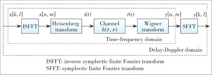
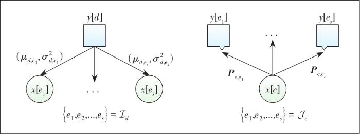
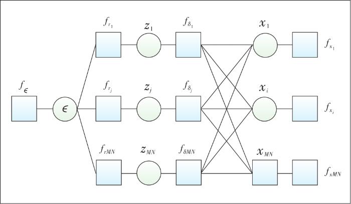
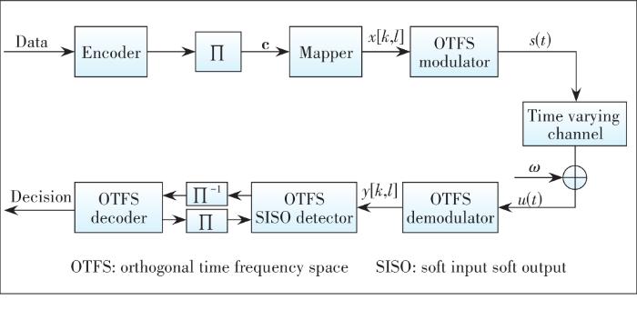
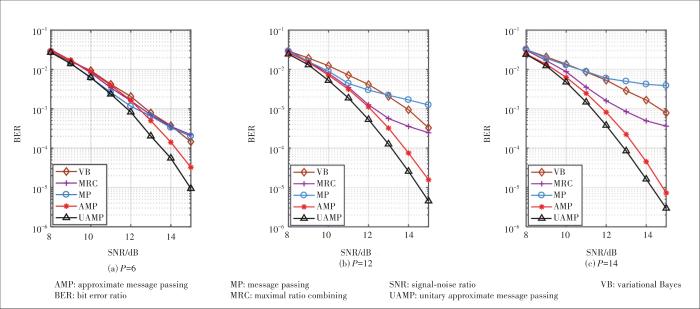
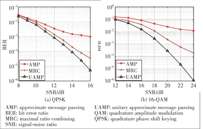
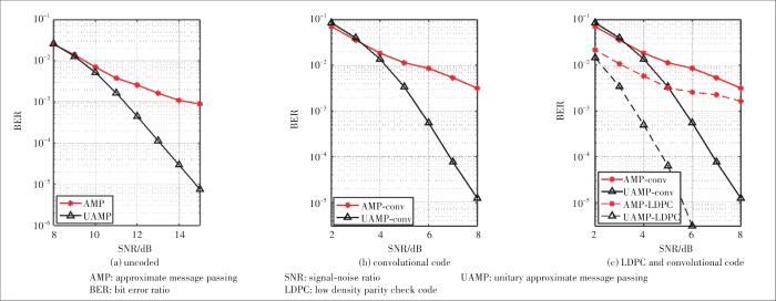
